Lecture 10: MLE and MAP

Additional links:

• Original class material

<< Previous lecture | Next lecture >>

---

todo clean

Probabilities in Machine Learning

In the ML lecture we said that a major assumption in Machine Learning is that there exists a (possibly stochastic) target function $f(x)$ such that $y=f(x)$ for any $x\in {\mathbb{R}}^d$, and such that the datasets

$$X=[x^1{x}^2\dots x^N]\in {\mathbb{R}}^{d\times N}$$ $$Y=[y^1{y}^2\dots y^N]\in {\mathbb{R}}^N$$

are generated by considering $N$ independent identically distributed (i.i.d.) samples $x^i\sim p(x)$, where $p(x)$ is the unknown distribution of the inputs, and considering $y^i=f(x^i)$ for any $i=1,\dots ,N$. When $f(x)$ is a stochastic function, we can consider the sampling process of $y^i$ as $y^i\sim p(y\Vert x^i)$ for any $i=1,\dots ,N$. In this setup, we can consider the decomposition

$$p(x,y)=p(y|x)p(x)$$

where $p(x,y)$ is the joint distribution, $p(x)$ is called prior distribution over $x\in {\mathbb{R}}^d$, while $p(y\Vert x)$ is the likelihood or posterior distribution of $y$ given $x$. With this framework, learning a Machine Learning model $f_{\theta }(x)\approx f(x)$ for any $x\sim p(x)$ with parameters $\theta \in {\mathbb{R}}^s$, can be reformulating as learning a parameterized distribution $p_{\theta }(y\Vert x)$ which maximizes the probability of observing $y$, given $x$.

Maximum Likelihood Estimation (MLE)

Intuitively, we would like to find parameters $\theta \in {\mathbb{R}}^s$ such that the probability of observing $Y=[y^1{y}^2\dots y^N]$ given $X=[x^1{x}^2\dots x^N]$ is as high as possible. Consequently, we have to solve the optimization problem

$${\theta }_{MLE}=\arg \underset{\theta \in {\mathbb{R}}^s}{\max }{p}_{\theta }(Y|X)$$

Which is usually called Maximum Likelihood Estimation (MLE), because the parameters ${\theta }_{MLE}$ are chosen such that they maximize the likelihood $p_{\theta }(Y\Vert X)$. Since $y^1,y^2,\dots ,y^N$ are independent under $p(y\Vert x)$,

$$p_{\theta }(Y|X)=p_{\theta }((y^1,y^2,\dots ,y^N)|X)=\prod _{i=1}^N{p}_{\theta }(y^i|X)$$

and since $y^i$ is independent with $x^j$ for any $j\ne i$, then

$$\prod _{i=1}^N{p}_{\theta }(y^i|X)=\prod _{i=1}^N{p}_{\theta }(y^i|x^i)$$

Consequently, \eqref{eq:mle_formulation1} becomes:

$${\theta }_{MLE}=\arg \underset{\theta \in {\mathbb{R}}^s}{\max }\prod _{i=1}^N{p}_{\theta }(y^i|x^i)$$

Since the logarithm function is monotonic, applying it to the optimization problem \eqref{eq:mle_formulation2} does not alterate its solution. Moreover, since for any function $f(x)$, $\arg {\max }_{x}f(x)=\arg {\min }_x-f(x)$, \eqref{eq:mle_formulation2} can be restated as

$${\theta }_{MLE}=\arg \underset{\theta \in {\mathbb{R}}^s}{\max }\prod _{i=1}^N{p}_{\theta }(y^i|x^i)=\arg \underset{\theta \in {\mathbb{R}}^s}{\min }-\log \prod _{i=1}^N{p}_{\theta }(y^i|x^i)=\arg \underset{\theta \in {\mathbb{R}}^s}{\min }\sum _{i=1}^N-\log p_{\theta }(y^i|x^i)$$

which is the classical formulation of an MLE problem. Note that in \eqref{eq:mle_formulation3}, the objective function has been decomposed into a sum over the datapoints $(x^i,y^i)$ for any $i$, as a consequence of the $x^i$ being i.i.d.. This formulation is similar to what we required in the previous lecture, implying that we can use SGD to (approximately) solve \eqref{eq:mle_formulation3}.

Gaussian Assumption

To effectively solve \eqref{eq:mle_formulation3}, we must explicitely define $p_{\theta }(y|x)$. A common assumption, which is true for most of the scenarios, is to consider

$$p_{\theta }(y|x)=\mathcal{N}(f_{\theta }(x),{\sigma }^{2}I)$$

where $\mathcal{N}(f_{\theta }(x),{\sigma }^{2}I)$ is a Gaussian distribution with mean $f_{\theta }(x)$ and variance ${\sigma }^{2}I$, with $f_{\theta }(x)$ a parametric deterministic function of $x$ while ${\sigma }^2$ is the variance of $p_{\theta }(y\Vert x)$, which depends on the informations we have on the relationship between $y$ and $x$ (it will be clearer in the following example).

An interesting property of the Gaussian distribution is that if $p_{\theta }(y\Vert x)=\mathcal{N}(f_{\theta }(x),{\sigma }^{2}I)$, then $y=f_{\theta }(x)+{\sigma }^{2}e$, where $e\sim \mathcal{N}(0,I)$ is a Standard Gaussian distribution.

To simplify the derivation below, assume that $d=1$, so that $X=[x^1{x}^2\dots x^N]\in {\mathbb{R}}^N$ and $x^i\in \mathbb{R}$ for any $i$. It is known that if $p_{\theta }(y\Vert x)=\mathcal{N}(f_{\theta }(x),{\sigma }^2)$, then

$$p_{\theta }(y|x)=\frac{1}{\sqrt{2\pi {\sigma }^2}}{e}^{\frac{(y-f_{\theta }(x){)}^2}{2{\sigma }^2}}$$

thus

$$-\log p_{\theta }(y|x)=\frac{1}{2}\log 2\pi +\frac{1}{2}\log {\sigma }^2+\frac{1}{2{\sigma }^2}(y-f_{\theta }(x){)}^2=\frac{1}{2}(y-f_{\theta }(x){)}^2+const.$$

Consequently, MLE with Gaussian likelihood becomes

$${\theta }_{MLE}=\arg \underset{\theta \in {\mathbb{R}}^s}{\min }\sum _{i=1}^N\frac{1}{2}(y^i-f_{\theta }(x^i){)}^2$$

which can be reformulated as a Least Squares problem

$${\theta }_{MLE}=\arg \underset{\theta \in {\mathbb{R}}^s}{\min }\frac{1}{2}||f_{\theta }(X)-Y|{|}_2^2$$

where $Y=[y^1{y}^2\dots y^N]$, while $f_{\theta }(X)=[f_{\theta }(x^1)f_{\theta }(x^2)\dots f_{\theta }(x^N)]$.

Polynomial Regression MLE

Now, consider a Regression model

$$f_{\theta }(x)=\sum _{j=1}^K{\varphi }_j(x){\theta }_j={\varphi }^T(x)\theta$$

and assume that

$$p_{\theta }(y|x)=\mathcal{N}({\varphi }^T(x)\theta ,{\sigma }^2)$$

Then, by \eqref{eq:MLE_gaussian},

$${\theta }_{MLE}=\arg \underset{\theta \in {\mathbb{R}}^K}{\min }\frac{1}{2}||\Phi (X)\theta -Y|{|}_2^2$$

where

$$\Phi (X)=[{\varphi }_1(X){\varphi }_2(X)\dots {\varphi }_K(X)]\in {\mathbb{R}}^{N\times K}$$

is the Vandermonde matrix associated with the vector $X$ and with feature vectors ${\varphi }_1,\dots ,{\varphi }_K$. Clearly, when ${\varphi }_j(x)=x^{j-1}$, the regression model $f_{\theta }(x)$ is a Polynomial Regression model and the associated Vandermonde matrix $\Phi (X)$ is the classical Vandermonde Matrix

$$\Phi (X)=\left[\begin{array}{ccccc}1& (x^1)& (x^1{)}^2& \dots & (x^1{)}^{K-1}\\ 1& (x^2)& (x^2{)}^2& \dots & (x^2{)}^{K-1}\\ ⋮& ⋮& ⋮& \dots & ⋮\\ 1& (x^N)& (x^N{)}^2& \dots & (x^N{)}^{K-1}\end{array}\right]\in {\mathbb{R}}^{N\times K}$$

Note that \eqref{eq:MLE_regression} defines a training procedure for a regression model. Indeed, it can be optimized by Gradient Descent (or its Stochastic variant), by solving

$$\{\begin{array}{l}{\theta }_0\in {\mathbb{R}}^K\\ {\theta }_{k+1}={\theta }_k-{\nabla }_{\theta }(-\log p_{{\theta }_k}(y|x))\end{array}$$

where

$${\nabla }_{\theta }(-\log p_{\theta }(y|x))={\nabla }_{\theta }\frac{1}{2}||\Phi (X)\theta -Y|{|}_2^2=\Phi (X{)}^T(\Phi (X)\theta -Y)$$

Direct solution by Normal Equations

Note that, since the learning problem is a Least Square problem of the form

$$\underset{\theta \in {\mathbb{R}}^K}{\min }\frac{1}{2}||\Phi (X)\theta -Y|{|}_2^2$$

then it can be solved directly by the Normal Equation method, i.e.

$${\theta }^{\ast }=(\Phi (X{)}^T\Phi (X){)}^{-1}\Phi (X{)}^{T}Y$$

this solution can be compared with the convergence point of Gradient Descent, to check the differences.

MLE + Flexibility = Overfit

In polynomial regression, the most important parameter the user has to set is the degree of polynomial, $K$. Indeed, when $K$ is low, the resulting model $f_{\theta }(x)$ will be pretty rigid (not flexible), with the implication that it can potentially be unable to capture the complexity of the data. On the opposite side, if $K$ is too large, the resulting model is too flexible, and we end up learning the noise. The former situation, which is called underfitting, can be easily diagnoised by looking at a plot of the resulting model with respect to the data (or, equivalently, by checking the accuracy of the model). Conversely, when the model is too flexible, we are in an harder scenario known as overfitting. In overfitting, the model is not understanding the knowledge of the data, but it is memorizing the training set, usually resulting in optimal training error and bad test prediction.

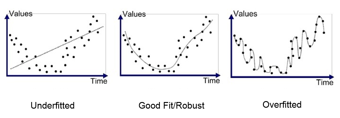
Ideally, when the data is generated by a noisy polynomial experiment, we would like to set $K$ as the real degree of such polynomial. Unfortunately, this is not always possible and indeed, spotting overfitting is the hardest issue to solve while working with Machine Learning.

Solving overfitting using the error plot

A common way to solve overfit, is to plot the error of the learnt model with respect to its complexity (i.e. the degree $K$ of the polynomial). In particular, for $K=1,2,\dots$, one can train a polynomial regressor $f_{\theta }(x)$ of degree $K$ over the training set $(X,Y)$ and compute the training error as the average absolute error of the prediction on the training set, i.e.

$${\mathcal{T}\mathcal{R}}_K=\frac{1}{N}||\Phi (X){\theta }^{\ast }-Y|{|}_2^2$$

and, for the same set of parameters, the test error

$${\mathcal{T}\mathcal{E}}_K=\frac{1}{N_{test}}||\Phi (X^{test}){\theta }^{\ast }-Y^{test}|{|}_2^2$$

If we plot the training and test error with respect to the different values of $K$, we will observe the following situation:

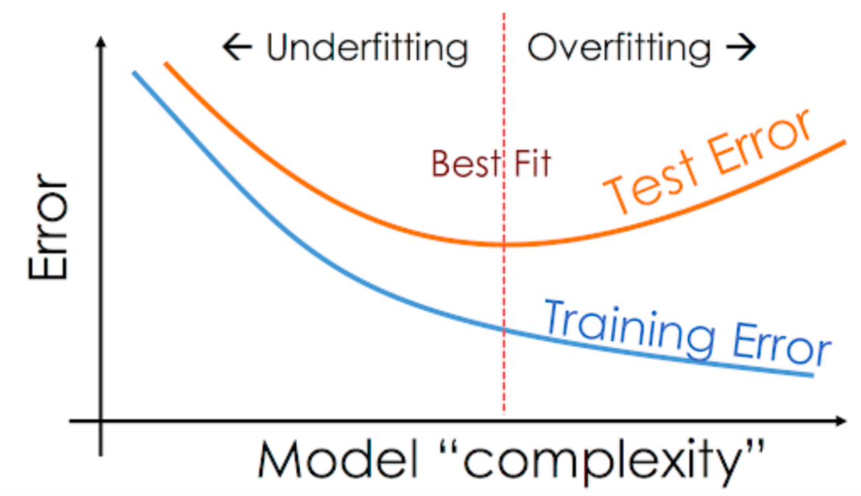
which will help us to find the correct parameter $K$, not suffering underfitting nor overfitting.

A better solution: Maximum A Posteriori (MAP)

A completely different approach to overfitting is to change the perspective and stop using MLE. The idea is to reverse the problem and, instead of searching parameters $\theta$ such that the probability of observing the outcomes $Y$ given the data $X$ is maximized, i.e. maximizing $p_{\theta }(y\Vert x)$, as in MLE, try to maximize the probability that the observed data is $(X,Y)$, given the parameters $\theta$. Mathematically, we are asked to solve the optimization problem

$${\theta }_{MAP}=\arg \underset{\theta \in {\mathbb{R}}^s}{\max }p(\theta |X,Y)$$

Since $p(\theta \Vert X,Y)$ is called posterior distribution, this method is usually referred to as **Maximum A Posteriori (MAP).

Bayes Theorem

A problem of MAP, is that it is non-trivial to find a formulation for $p(\theta \Vert X,Y)$. Indeed, if with MLE the Gaussian assumption made sense, as a consequence of the hypothesis that the observations $y$ are obtained by corrupting a deterministic function of $x$ by Gaussian noise, this does not hold true for MAP, since in general the generation of $X$ given $Y$ is not Gaussian.

Luckily, we can express the posterior distribution $p(\theta \Vert X,Y)$ in terms of the likelihood $p(Y\Vert X,\theta )$ (which we know to be Gaussian) and the prior $p(\theta )$, as a consequence of Bayes Theorem. Indeed, it holds

$$p(\theta |X,Y)=\frac{p(Y|X,\theta )p(\theta )}{p(Y|X)}$$

Gaussian assumption on MAP

For what we observed above, the posterior distribution $p(\theta \Vert X,Y)$ can be rewritten as a function of the likelihood $p(Y\Vert X,\theta )$ and the prior $p(\theta )$. Thus, \eqref{eq:MAP_formulation1} can be rewritten as

$${\theta }_{MAP}=\arg \underset{\theta \in {\mathbb{R}}^s}{\max }p(\theta |X,Y)=\arg \underset{\theta \in {\mathbb{R}}^s}{\max }\frac{p(Y|X,\theta )p(\theta )}{p(Y|X)}$$

With the same trick we used in MLE, we can change it to a minimum point estimation by changing the sign of the function and by taking the logarithm. We obtain,

$${\theta }_{MAP}=\arg \underset{\theta \in {\mathbb{R}}^s}{\max }\frac{p(Y|X,\theta )p(\theta )}{p(Y|X)}=\arg \underset{\theta \in {\mathbb{R}}^s}{\min }-\log p(Y|X,\theta )-\log p(\theta )$$

where we removed $p(Y|X)$ since it is constant in $\theta$.

Since $x^1,\dots ,x^N$ are i.i.d. by hypothesis and by following the same procedure of MLE, we can split \eqref{eq:MAP_formulation3} into a sum over datapoints, as

$${\theta }_{MAP}=\arg \underset{\theta \in {\mathbb{R}}^s}{\min }-\log \prod _{i=1}^{N}p(y^i|x^i,\theta )-\log p(\theta )=\arg \underset{\theta \in {\mathbb{R}}^s}{\min }\sum _{i=1}^N-\log p(y^i|x^i,\theta )-\log p(\theta )$$

Now, if we assume that $p(y^i\Vert x^i,\theta )=\mathcal{N}(f_{\theta }(x^i),{\sigma }^{2}I)$, the same computation we did in MLE implies

$${\theta }_{MAP}=\arg \underset{\theta \in {\mathbb{R}}^s}{\min }\sum _{i=1}^N\frac{1}{2{\sigma }^2}(f_{\theta }(x^i)-y^i{)}^2-\log p(\theta )$$

To complete the derivation, we have to rewrite $p(\theta )$ in a meaningful way, to be able to perform the optimization. To do that, it is common to assume that $p(\theta )=\mathcal{N}(0,{\sigma }_{\theta }^{2}I)$, a Gaussian distribution with zero mean and variance ${\sigma }_{\theta }^2$. Under this assumption,

$$-\log p(\theta )=\frac{1}{2{\sigma }_{\theta }^2}||\theta |{|}_2^2$$

and consequently

$${\theta }_{MAP}=\arg \underset{\theta \in {\mathbb{R}}^s}{\min }\sum _{i=1}^N\frac{1}{2{\sigma }^2}(f_{\theta }(x^i)-y^i{)}^2+\frac{1}{2{\sigma }_{\theta }^2}||\theta |{|}_2^2=\arg \underset{\theta \in {\mathbb{R}}^s}{\min }\frac{1}{2}||f_{\theta }(X)-Y|{|}_2^2+\frac{\lambda }{2}||\theta |{|}_2^2$$

where $\lambda =\frac{{\sigma }^2}{{\sigma }_{\theta }^2}$ is a positive parameter, usually called regularization parameter. This equation is the final MAP loss function under Gaussian assumption for both $p(Y\Vert X,\theta )$ and $p(\theta )$. Clearly, it is another Least Squares problem which can be solved by Gradient Descent or Stochastic Gradient Descent.

When $f_{\theta }(x)$ is a polynomial regression model, $f_{\theta }(X)=\Phi (X)\theta$, then

$${\theta }_{MAP}=\arg \underset{\theta \in {\mathbb{R}}^s}{\min }\frac{1}{2}||\Phi (X)\theta -Y|{|}_2^2+\frac{\lambda }{2}||\theta |{|}_2^2$$

can be also solved by Normal Equations, as

$${\theta }_{MAP}=(\Phi (X{)}^T\Phi (X)+\lambda I{)}^{-1}\Phi (X{)}^{T}Y$$

Ridge Regression and LASSO

When the Gaussian assumption is used for both the likelihood $p(Y\Vert X,\theta )$ and the prior $p(\theta )$, the resulting MAP is usually called Ridge Regression in the literature. On the contrary, if $p(Y\Vert X,\theta )$ is Gaussian and $p(\theta )=Lap(0,{\sigma }_{\theta }^2)$ is a Laplacian distribution with mean 0 and variance ${\sigma }_{\theta }^2$, then

$$p(\theta )=\frac{1}{2{\sigma }_{\theta }^2}{e}^{-\frac{|\theta |}{{\sigma }_{\theta }^2}}$$

and consequently (prove it by exercise)

$${\theta }_{MAP}=\arg \underset{\theta \in {\mathbb{R}}^s}{\min }\frac{1}{2}||\Phi (X)\theta -Y|{|}_2^2+\lambda ||\theta |{|}_1$$

the resulting model is called LASSO, and it is the basis for most of the classical, state-of-the-art regression models.

---

• Homework assignments
• Lab lecture list