Lecture 9: Linear and Polynomial Regression

Additional links:

• Original class material

<< Previous lecture | Next lecture >>

---

todo clean

Regression in Machine Learning

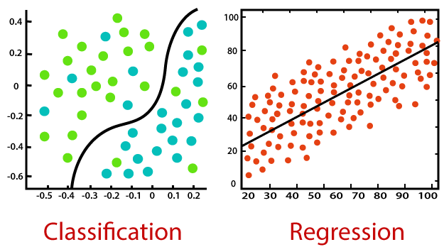
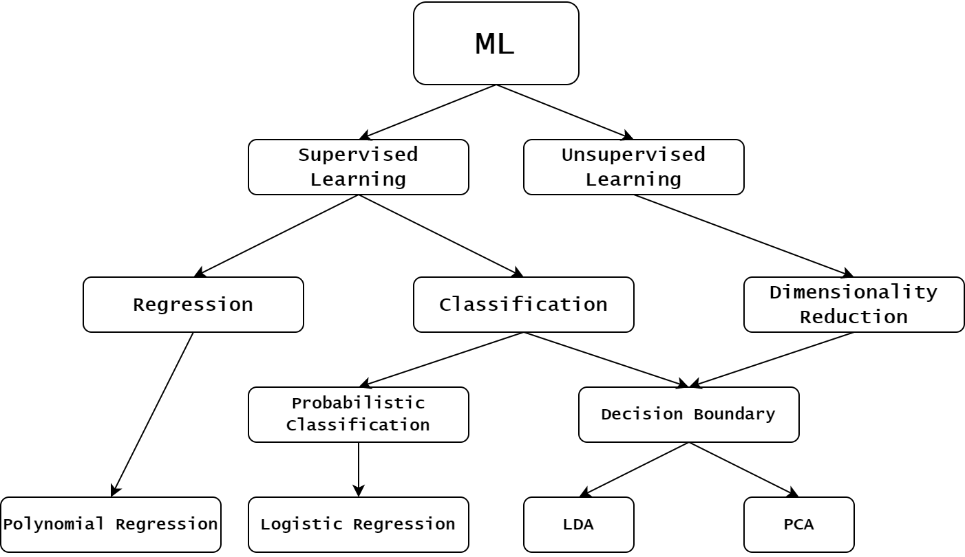Regression in a group of supervised learning techniques, alternative to classification. In classification, given a datapoint $x\in {\mathbb{R}}^d$, the task was to learn a model $y=f_{\theta }(x)$ such that $y$ represents one of the $K$ possible classes in which $x$ lies. On the other side, a Machine Learning problem is a Regression when the target variable $y\in \mathbb{R}$ is a continuous variable, and the task is to approximately interpolate between the $y$ values, with the intent of being able to predict new outcome of $y$ when a new $x$ is given as input. A part from that, the computation procedure to define a regression model is similar to the procedure required for a classification model. Indeed, let $f_{\theta }(x)$ be a parametric function of $x\in {\mathbb{R}}^d$, parameterized by $\theta \in {\mathbb{R}}^s$. Given a dataset

$$X=[x^1{x}^2\dots x^N]\in {\mathbb{R}}^{d\times N}$$ $$Y=[y^1{y}^2\dots y^N]\in {\mathbb{R}}^N$$

the task is to train the model such that $f_{\theta }(x^i)\approx y^i$ for any $i=1,\dots ,N$. Clearly, this is done by solving the optimization problem

$${\theta }^{\ast }=\arg \underset{\theta \in {\mathbb{R}}^s}{\min }\ell (\theta ;X,Y)$$

where the specific form of the loss function $\ell (\theta ;X,Y)$ will be given in the next post. When $d>1$, $f_{\theta }(x)$ is called multivariate regression model, while if $d=1$, $f_{\theta }(x)$ is an univariate regression model. For simplicity, from now on we will work with univariate regression models, where $x^i\in \mathbb{R}$ for any $i=1,\dots ,N$, and consequently $X=[x^1{x}^2\dots x^N]\in {\mathbb{R}}^N$.

Linear Regression

The simplest regression model we can think of is the Linear Regression Model, defined as

$$f_{\theta }(x)={\theta }_1+{\theta }_{2}x={\theta }^T\hat{x}$$

where $\theta =[{\theta }_1,{\theta }_2{]}^T$ and $\hat{x}=[1,x{]}^T$. When $\theta$ is optimized, it defines a straight line approximating the data. Clearly, the resulting model will be correct if and only if the real function $y=f(x)$ generating the data is linear. Unfortunately, even in situations where $f(x)$ can be considered linear, the collected data $y$ is always corrupted by noise, which consequently breaks the linearity.

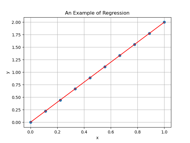
Consider for example a situation where $y=f(x)=2x$ is the model generating the data. The noiseless data $y$, together with the line generated by the prediction model $f_{\theta }(x)$, in that situation will look like that

Unfortunately, since the data is always corrupted by noise, the collected data will be more like

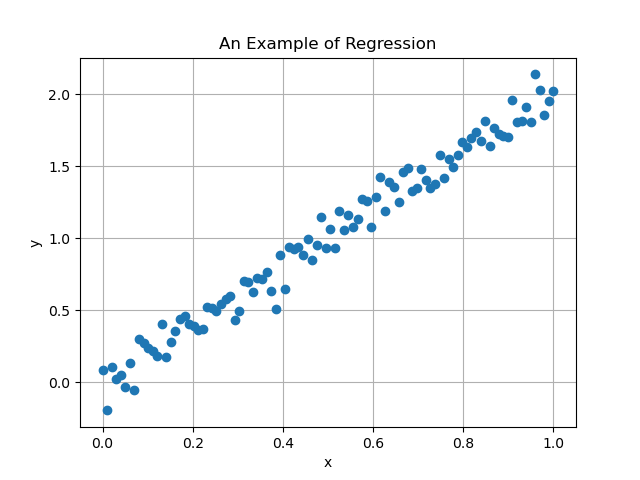
In this scenario, if $f_{\theta }(x)={\theta }^T\hat{x}$ as in the assumption above, then we hope to find parameters $\theta$ such that the resulting line will be close to the original one (first figure), someway ignoring the noise present in the data. Luckily, at least when the noise is Gaussian distributed, it usually does the job. Indeed the resulting linear regression model from the image above is 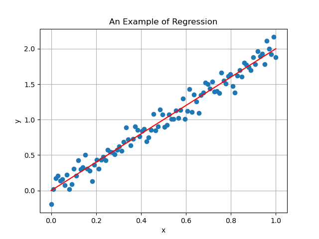which is almost equal to the real line from the first image.

Polynomial Regression

In most of real life scenario, the linear regression model is too rigid to correctly approximate the data. Indeed, suppose to collect a dataset like 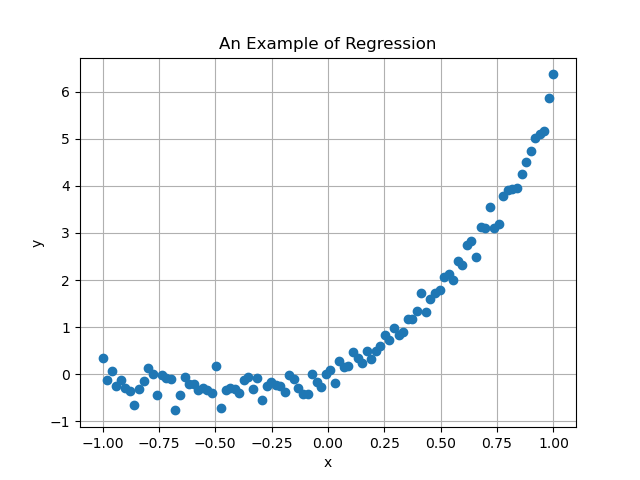where it is clear that no straight line is able to correctly approximate it. Indeed, if we try to approximate it with a linear regression model, we obtain 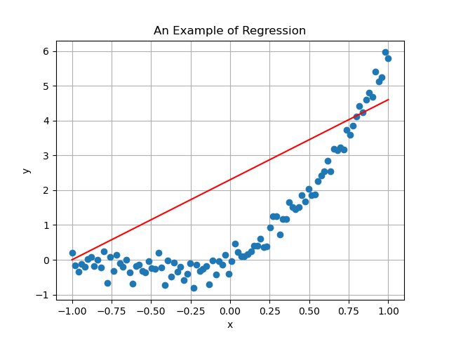When this is the case, it is required to define a more flexible model.

Given a number $K>0$, define the regression model

$$f_{\theta }(x)=\sum _{j=0}^K{\varphi }_j(x){\theta }_j$$

where the functions ${\varphi }_1,{\varphi }_2,\dots ,{\varphi }_K$ are called feature vectors. Note that, for $K=2$ and ${\varphi }_0(x)=1$, ${\varphi }_1(x)=x$, we recover the linear regression model $f_{\theta }(x)={\theta }_1+{\theta }_{2}x$. For different values of $K$ and different feature vectors ${\varphi }_j(x)$, we get different regression model.

Note that, if $\theta =[{\theta }_1,{\theta }_2,\dots ,{\theta }_K{]}^T$ and $\varphi (x)=[{\varphi }_1(x),{\varphi }_2(x),\dots ,{\varphi }_K(x){]}^T$, then

$$f_{\theta }(x)={\varphi }^T(x)\theta$$

which implies that $f_{\theta }(x)$ is a linear function in $\theta$, for any choice of ${\varphi }_j(x)$.

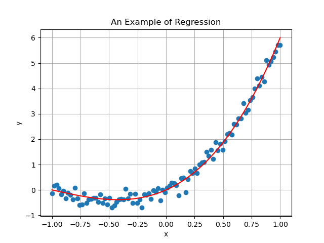
A classical choice for the feature vector, is ${\varphi }_j(x)=x^{j-1}$. In this way, for a given $K>0$, $\varphi (x)$ represents the vector of the first $K$ monomial in $x$, i.e.

$$\varphi (x)=[1,x,x^2,\dots ,x^{K-1}{]}^T$$

and $f_{\theta }(x)$ is a $K-1$-th degree polynomial. For this reason, $f_{\theta }(x)$ is called polynomial regression model for this choice of ${\varphi }_j(x)$. To show the improvement of a polynomial regression model against a linear model, this is the resulting model when we use a polynomial regression model of degree 3 on the data above: To understand how to train the parameters $\theta$ of a linear / polynomial regression model, we have to move to the next post.

---

• Homework assignments
• Lab lecture list