Lecture 11: Logistic regression

Additional links:

• Original class material

<< Previous lecture |

---

todo clean

Binary Classification

Assume we are working in a binary classification setup, i.e. where the number of classes $K=2$. In this case, we can always represent the two classes as $y=0$ and $y=1$.

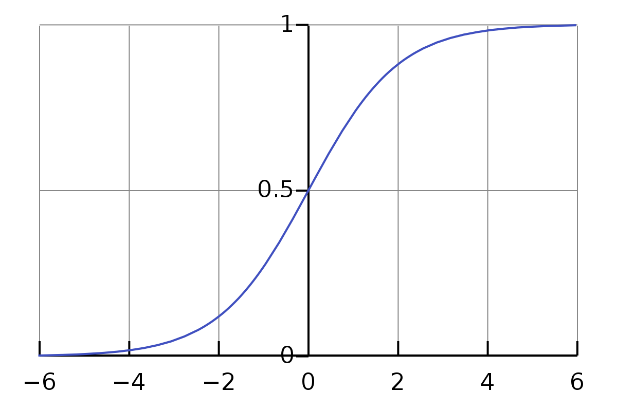
Consequently, we can develop a classification algorithm by defining a model $f_w(x)$ such that $f_w:{\mathbb{R}}^d\to [0,1]$ and interpret the outcome of $f_w(x)$ as the probability that $y=1$. Thus, if $f_w(x)=0$, then our model predict that there are zero chances of $x$ being classified as $1$, meaning that $x$ should be a 0. If $f_w(x)=1$, then $x$ will be classified as 1, while if $f_w(x)=0.5$ then the model is not able to correctly identify the class of $x$, since the chances of being $1$ are 50%.

An interesting feature of $f_w(x)$ is that it turns a discontinuous task (i.e. mapping a real vector $x$ to a discrete value $y$) into a continuous problem. The discreteness of the outcome is then recovered by mapping $f_w(x)$ to 1 if $f_w(x)>0.5$, to 0 is $f_w(x)<0$. In formula, a datapoint $x\in {\mathbb{R}}^d$ will be classified as:

$$\{\begin{array}{l}1\text{if }{f}_w(x)>0.5\\ 0\text{if }{f}_w(x)<0.5\end{array}$$

What is logistic regression?

Logistic Regression is a widely known, beginner-level, binary classification algorithm based on the probabilistic approach framework. The idea is simple: consider a dataset

$$X=[x^1{x}^2\dots x^N]\in {\mathbb{R}}^{d\times N}$$

and consider a linear function with unknown parameters $w=(w_0,w_1,\dots ,w_d)\in {\mathbb{R}}^{d+1}$ over each of the datapoints $w_0+w_1{x}_1^i+\dots w_d{x}_d^i$. This operation can be rewritten as $[1;x^i{]}^{T}w$. Consequently, define the extended dataset $\hat{X}$, computed adding a 1 to each datapoint, i.e.

$$\hat{X}=[{\hat{x}}^1{\hat{x}}^2\dots {\hat{x}}^N]\in {\mathbb{R}}^{(d+1)\times N}$$

where

$$\hat{x}=[1,x_1,x_2,\dots ,x_d{]}^T.$$

Then, for any $i=1,\dots ,N$, consider the model

$$f_w(x)=\sigma ({\hat{x}}^{T}w)$$

where $w\in {\mathbb{R}}^{d+1}$ is the weight vector, and $\sigma (z)$ is the sigmoid function, defined as

$$\sigma (z)=\frac{1}{1+e^{-z}}$$

whose scope is to squeeze the real axis to the domain $[0,1]$ (to get the probabilistic interpretation). Since the output of $f_w(x)$ is continuous, it is natural to select, as loss function, the Mean Squared Error, as defined previously. Indeed, the loss function becomes

$$\ell (w;\mathbb{D})=\frac{1}{N}\sum _{i=1}^{N}MSE(f_w(x_i),y_i)$$

and the training procedure is

$$w^{\ast }=\arg \underset{w\in {\mathbb{R}}^n}{\min }\ell (w;\mathbb{D})$$

which can be done by Gradient Descent (or, alternatively, Stochastic Gradient Descent), whose iteration is

$$w_{k+1}=w_k-{\alpha }_k{\nabla }_w\ell (w_k;\mathbb{D})$$

for which we are required to compute

$${\nabla }_w\ell (w;\mathbb{D})=\frac{1}{N}\sum _{i=1}^N{\nabla }_{w}MSE(f_w(x_i),y_i).$$

Since

$$MSE(f_w(x_i),y_i)=\frac{1}{2}(f_w(x_i)-y_i{)}^2$$

then

$${\nabla }_{w}MSE(f_w(x_i),y_i)={\nabla }_w(\frac{1}{2}(f_w(x_i)-y_i{)}^2)={\nabla }_w{f}_w(x_i{)}^T(f_w(x_i)-y_i)$$

since $f_w(x_i)=\sigma ({\hat{x}}_i^{T}w)$ by \eqref{eq:model_definition}, then the chain rule implies that

$${\nabla }_w{f}_w(x_i)={\sigma }^{\prime }({\hat{x}}_i^{T}w){\hat{x}}_i^T.$$

An interesting feature of $\sigma (z)$ is that ${\sigma }^{\prime }(z)=\sigma (z)(1-\sigma (z))$, impliying that

$${\nabla }_w{f}_w(x_i)=\sigma ({\hat{x}}_i^{T}w)(1-\sigma ({\hat{x}}_i^{T}w)){\hat{x}}_i^T$$

and

$${\nabla }_{w}MSE(f_w(x_i),y_i)=\sigma ({\hat{x}}_i^{T}w)(1-\sigma ({\hat{x}}_i^{T}w)){\hat{x}}_i^T(f_w(x_i)-y_i)$$

which finally leads to

$$w_{k+1}=w_k-\frac{{\alpha }_k}{N}\sum _{i=1}^N\sigma ({\hat{x}}_i^{T}w)(1-\sigma ({\hat{x}}_i^{T}w)){\hat{x}}_i^T(f_w(x_i)-y_i)$$

which converges to the solution of \eqref{eq:training_procedure} for $k\to \infty$.

Python Implementation

Before we can start with the implementation notes, observe that we can do some operations to simplify the coding and the efficiency of it. Indeed, given the dataset $\hat{X}=[{\hat{x}}^1{\hat{x}}^2\dots {\hat{x}}^N]\in {\mathbb{R}}^{d\times N}$, define

$$f_w(\hat{X})=[f_w({\hat{x}}^1)f_w({\hat{x}}^2)\dots f_w({\hat{x}}^N)]\in {\mathbb{R}}^N$$

and

$$Y=[y^1{y}^2\dots y^N{]}^T\in {\mathbb{R}}^N$$

Consequently, we can re-write \eqref{eq:loss_function} as

$$\ell (w;\mathbb{D})=\frac{1}{N}\sum _{i=1}^N\frac{1}{2}(f_w(x^i)-y^i{)}^2=\frac{1}{2N}||f_w(\hat{X})-Y|{|}_2^2$$

and, by following the same procedure we did before, we get to the compact form of \eqref{eq:final_GD_iteration}:

$$w_{k+1}=w_k-\frac{{\alpha }_k}{N}{\hat{X}}^T(\sigma ({\hat{X}}^{T}w)\odot (1-\sigma ({\hat{X}}^{T}w))\odot (f_w(\hat{X})-Y))$$

where $\odot$ is the element-wise multiplication. To check that the shapes in Equation \eqref{eq:final_GD_iteration_compact} are correct, let’s do a sanity check:

• $\hat{X}$ has shape $k\times N$, where $k=d+1$ in this case;
• $w$ has shape $k\times 1$ by definition, then ${\hat{X}}^{T}w$ has shape $N\times 1$;
• $\sigma (\cdot )$ does not affect the shape of the input, then $\sigma ({\hat{X}}^{T}w)\odot (1-\sigma ({\hat{X}}^{T}w))$ has shape $N\times 1$;
• Both $f_w(\hat{X})$ and $Y$ have shape $N\times 1$, then $f_w(\hat{X})-Y$ has shape $N\times 1$.
• Consequently, $\sigma ({\hat{X}}^{T}w)\odot (1-\sigma ({\hat{X}}^{T}w))\odot (f_w(\hat{X})-Y)$ has shape $N\times 1$ because of the element-wise multiplication;
• Finally, ${\hat{X}}^T(\sigma ({\hat{X}}^{T}w)\odot (1-\sigma ({\hat{X}}^{T}w))\odot (f_w(\hat{X})-Y))$ has shape $k\times 1$, which is the same shape of $w_k$, then the computation is correct.

Equation \eqref{eq:final_GD_iteration_compact} is what we are going to implement.

Data Loading and Pre-processing

We are going to test logistic regression on a simulated dataset from the library sklearn. Loading it into memory is very easy:

import numpy as np
import matplotlib.pyplot as plt
from sklearn.datasets import make_classification
 
# Load data
X, Y = make_classification(n_samples=500, n_features=2, n_redundant=0, n_informative=1, 
                            n_clusters_per_class=1)
X = X.T # To make it d x N
 
# Check the shape
print(f"Shape of X: {X.shape}")
print(f"Shape of Y: {Y.shape}")
 
# Memorize the shape
d, N = X.shape
 
# Add dimension on Y
Y = Y.reshape((N, 1))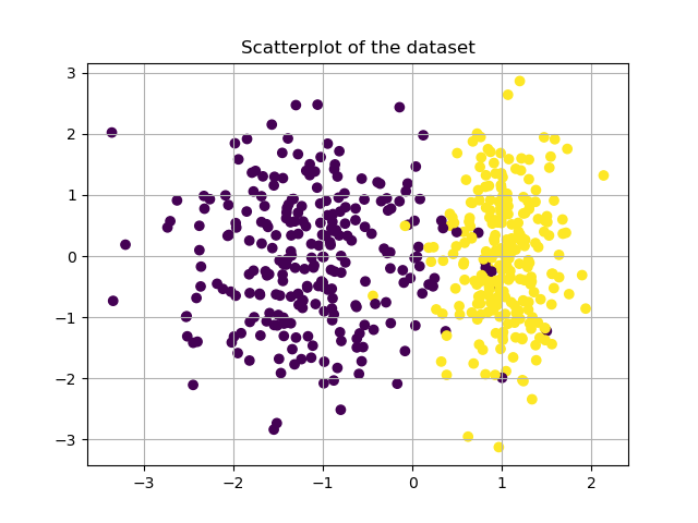

To conclude the data loading step, we need to build the $\hat{X}$ dataset from above. This can be simply done by

# Create Xhat
Xhat = np.concatenate((np.ones((N,1)), X), axis=0)

Build the model

Remember that

$$f_w(\hat{x})=\sigma ({\hat{x}}^{T}w)$$

thus, we need to define the sigmoid function $\sigma (z)$.

# Define sigmoid
def sigmoid(x):
    ...

The results of the application of $\hat{x}$ on $f_w(\hat{x})$ is not hard to compute.

# Compute the value of f
def f(w, xhat):
    ...

Training

To perform the training, it is sufficient to implement the loss function and its gradient, which can be simply done by following the formulas above

# Value of the loss
def ell(w, X, Y):
    ...
 
# Value of the gradient
def grad_ell(w, X, Y):
    ...

After training, the prediction over new data can be simply done by

def predict(w, X, treshold=0.5):
    ...

Results

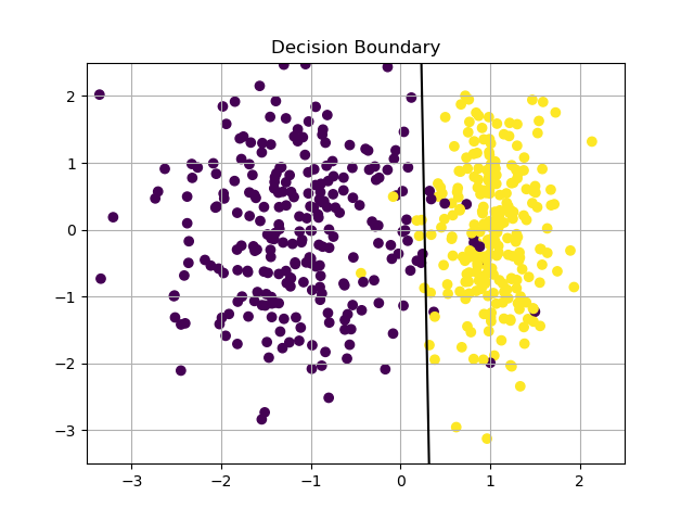
The result is a $(d+1)$-ple of weights $w=(w_0,w_1,\dots ,w_d)$ such that $f_w(x)=\sigma ({\sum }_{i=0}^d{w}_i{x}_i)$. When $d=2$, the term inside of the sigmoid is the equation of a straight line $w_0+w_1{x}_1+w_2{x}_2=0$, which can be re-written in explicit form as

$$x_2=-\frac{w_1}{w_2}{x}_1-\frac{w_0}{w_2}$$

which is the decision boundary for the classification problem. Here it is a plot of the resulting classifier.

Extension to $K>2$ case

If the number of classes $K$ is bigger than 2, logistic regression can still be applied, with slight modifications. In particular, let $K>2$ be the number of classes $\mathcal{C}=\{C_1,\dots ,C_K\}$. Then, we define $Y$ to be a $K\times N$ matrix,

$$Y=[y^1{y}^2\dots y^N]\in {\mathbb{R}}^{K\times N}$$

where $y^i=[y_1^i,y_2^i,\dots ,y_K^i]\in {\mathbb{R}}^K$ is a vector of probabilities (i.e. $y_k^i\in [0,1]$ for any $i=1,\dots ,N$ and $k\in 1,\dots ,K$) summing to one, i.e.

$$\sum _{k=1}^K{y}_k^i=1\forall i=1,\dots ,N$$

Intuitively, $y_k^i$ represents the probability the $x^i$ is a member of the class $C_k$. To enforce the condition \eqref{eq:summing_to_one}, it is mandatory to set

$$f_w(x)=softmax({\hat{x}}^{T}w)$$

where $softmax(z)$ is defined as

$$softmax(z{)}_i=\frac{e^{z_i}}{{\sum }_{j=1}^K{e}^{z_j}}$$

such that

$$\sum _{i=1}^{K}softmax(z{)}_i=1$$

Note that, in the multi-class scenario, the weights are $d\times K$ matrices, so that $X^{T}W$ is an $N\times K$ matrix.

---

• Homework assignments
• Lab lecture list