Lecture 7: Optimization with Gradient Descent

Additional links:

• Original class material

<< Previous lecture | Next lecture >>

---

todo clean

Introduction to Optimization

Consider a general continuous function $f:{\mathbb{R}}^n\to \mathbb{R}$. Given a set of admissible solutions $\Omega \subseteq {\mathbb{R}}^n$, an optimization problem is a problem of the form

$$\underset{x\in \Omega }{\min }f(x)$$

If $\Omega ={\mathbb{R}}^n$, we say that the optimization is unconstrained. If $\Omega \subset {\mathbb{R}}^n$, the problem is constrained. In this first part, we will always assume $\Omega ={\mathbb{R}}^n$, i.e. the unconstrained setup.

Convexity

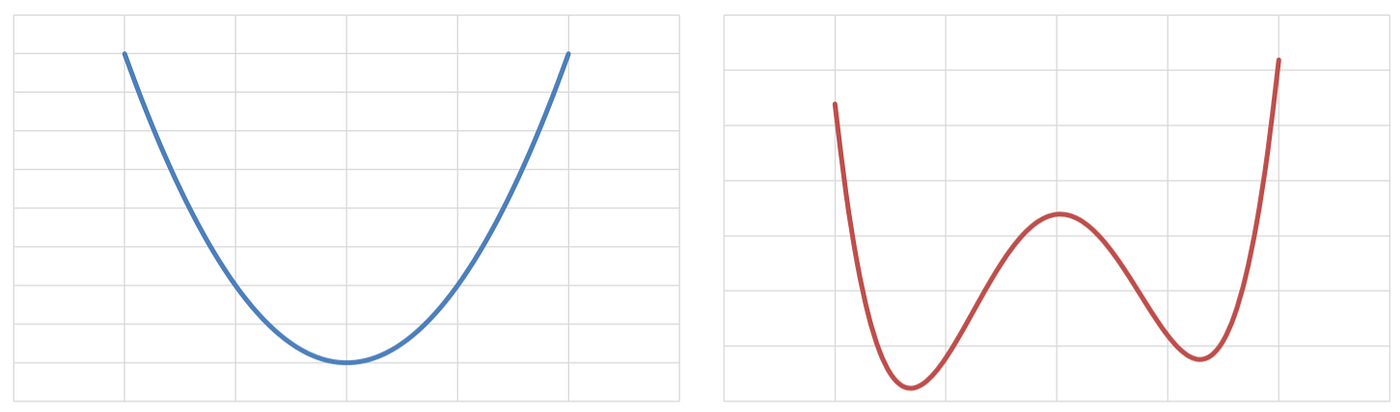
A common assumption in optimization is the convexity. By definition, a function $f:{\mathbb{R}}^n\to \mathbb{R}$ is convex if

$$f(t{x}_1+(1-t)x_2)\le tf(x_1)+(1-t)f(x_2)\forall x_1,x_2\in {\mathbb{R}}^n,\forall t\in [0,1]$$

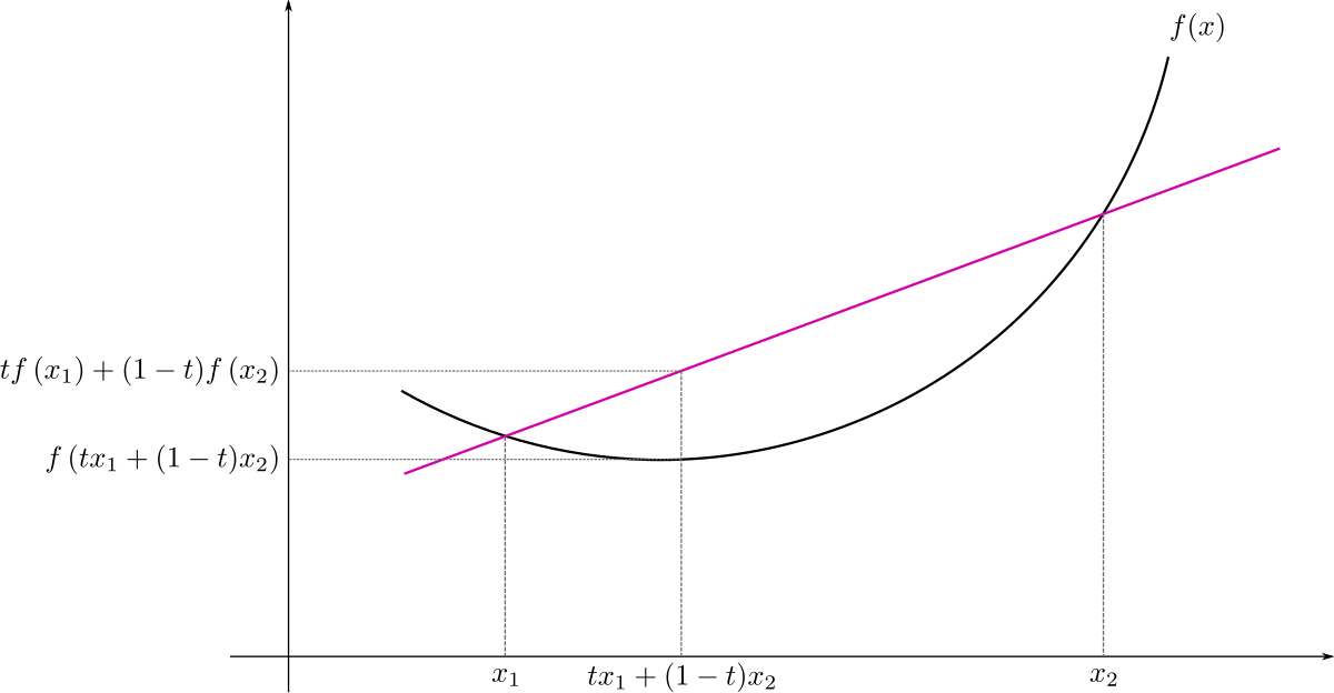
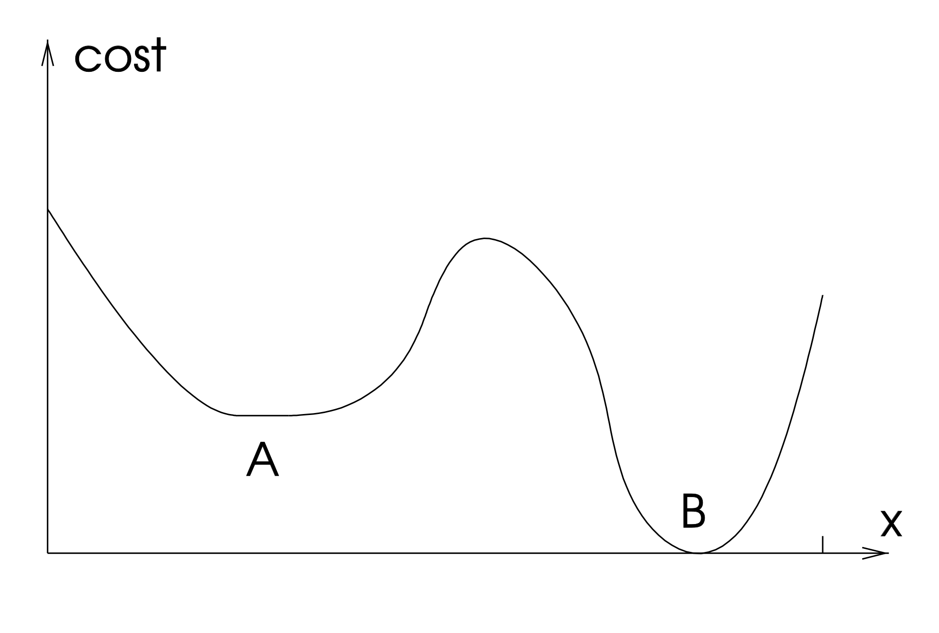
The importance of convex functions in optimization is that if $f(x)$ is convex, than every minimum point $x^{\ast }$ of $f(x)$ is a global minimum and the set of global minima is connected (the $n$-dimensional extension of the concept of interval). On the other side, if a function is non-convex (NOTE: the opposite of convex is not concave), then there can be multiple distinct minimum points, some of which are local minimum while others are global minimum. Since in ML applications we want to find global minima, and discriminating between local and global minima of a function is an NP-hard problem, having convexity is a good thing.

First-order conditions

Most of the algorithms to find the minimum points of a given function $f(x)$ are based on the following property:

First-order sufficient condition: If $f:{\mathbb{R}}^n\to \mathbb{R}$ is a continuously differentiable function and $x^{\ast }\in {\mathbb{R}}^n$ is a minimum point of $f(x)$, then $\nabla f(x^{\ast })=0$.

Moreover, it holds

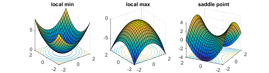
First-order necessary condition: If $f:{\mathbb{R}}^n\to \mathbb{R}$ is a continuously differentiable function and $\nabla f(x^{\ast })=0$ for $x^{\ast }\in {\mathbb{R}}^n$, then $x^{\ast }$ is either a (local) minimum, a (local) maximum or a saddle point of $f(x)$.

Consequently, we want to find a point $x^{\ast }\in {\mathbb{R}}^n$ such that $\nabla f(x^{\ast })=0$. Those points are called stationary points of $f(x)$.

Gradient descent (GD)

The most common algorithm to solve optimization problems is the so-called Gradient Descent (GD). It is an iterative algorithm, i.e. an algorithm that iteratively updates the estimate of the solution, converging to the correct solution after infinite steps, such that, at each iteration, the successive estimate is computed by moving in the direction of maximum decreasing of $f(x)$: $-\nabla f(x)$. Specifically,

$$x_{k+1}=x_k-{\alpha }_k\nabla f(x_k)k=0,1,\dots$$

where the initial iterate, $x_0\in {\mathbb{R}}^n$, is given as input and the step-size (equivalently, learning rate) ${\alpha }_k>0$ controls the decay rapidity of $f(x)$ for any $k\in \mathbb{N}$.

Choice the initial iterate

The Gradient Descent (GD) algorithm, always require the user to input an initial iterate $x_0\in {\mathbb{R}}^n$. Theoretically, since GD has a global convergence proprerty, for any $x_0$ it will always converge to a stationary point of $f(x)$, i.e. to a point such that $\nabla f(x)=0$.

If $f(x)$ is convex, then every stationary point is a (global) minimum of $f(x)$, implying that the choice of $x_0$ is not really important, and we can always use $x_0=0$. On the other side, when $f(x)$ is not convex, we have to choose $x_0$ such that it is as close as possible to the right stationary point, to increase the chances of getting to that. If an estimate of the correct minimum point is not available, we will just consider $x_0=0$ to get to a general local minima.

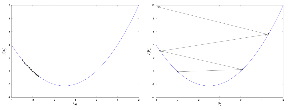
Step Size

Choosing the step size is the hardest component of gradient descent algorithm. Indeed, if ${\alpha }_k$ is too small, there is a chance we never get to the minimum, getting closer and closer without reaching it. Moreover, we can easily get stuck on local minima when the objective function is non convex. On the contrary, if ${\alpha }_k$ is too large, there is a chance we get stuck, bouncing back and forth around the minima.

Backtracking

Choosing the right step-size at each iteration is non-trivial. Indeed, convergence of Gradient Descent methods is only guaranteed if the step-size ${\alpha }_k$ satisfies, for any $k\in \mathbb{N}$, some conditions known as Wolfe Conditions:

• Sufficient decrease: $f(x_k-{\alpha }_k\nabla f(x_k))\le f(x_k)-c_1{\alpha }_k\Vert \nabla f(x_k){\Vert }_2^2$;
• Curvature condition: $\nabla f(x_k{)}^T\nabla f(x_k-{\alpha }_k\nabla f(x_k))\le c_2\Vert \nabla f(x_k){\Vert }_2^2$; with $0<c_1<c_2<1$.

Luckily, those conditions are automatically satisfied if ${\alpha }_k$ is chosen by the backtracking algorithm. The idea of this algorithm is to start from an initial guess for ${\alpha }_k$, and then reducing it as ${\alpha }_k\leftarrow \tau {\alpha }_k$ with $\tau <1$ until the sufficient decrease condition is satisfied. A Python implementation for the backtracking algorithm can be found in the following.

import numpy as np
 
def backtracking(f, grad_f, x):
    """
    This function is a simple implementation of the backtracking algorithm for
    the GD (Gradient Descent) method.
    
    f: function. The function that we want to optimize.
    grad_f: function. The gradient of f(x).
    x: ndarray. The actual iterate x_k.
    """
    alpha = 1
    c = 0.8
    tau = 0.25
    
    while f(x - alpha * grad_f(x)) > f(x) - c * alpha * np.linalg.norm(grad_f(x), 2) ** 2:
        alpha = tau * alpha
        
        if alpha < 1e-3:
            break
    return alpha

Stopping Criteria

The gradient descent is an iterative algorithm, meaning that it iteratively generates new estimates of the minima, starting from $x_0$. Theoretically, after infinite iterations, we converge to the solution of the optimization problem but, since we cannot run infinite iterations, we have to find a way to tell the algorithm when its time to stop. A convergence condition for an iterative algorithm is called stopping criteria.

Remember that gradient descent aim to find stationary point. Consequently, it would make sense to use the norm of the gradient as a stopping criteria. In particular, it is common to check if the norm of the gradient on the actual iterate is below a certain tollerance and, if so, we stop the iterations. In particular

Stopping criteria 1: Given a tollerance $to{l}_f$, for any iterate $x_k$, check whether or not $\Vert \Vert \nabla f(x_k)\Vert \Vert <to{l}_f\Vert \Vert \nabla f(x_0)\Vert \Vert$. If so, stop the iterations.

Unfortunately, this condition alone is not sufficient. Indeed, if the function $f(x)$ is almost flat around its minimum, then $\Vert \Vert \nabla f(x_k)\Vert \Vert$ will be small even if $x_k$ will be far from the true minimum.

Consequently, its required to add another stopping criteria.

Stopping criteria 2: Given a tollerance $to{l}_x$, for any iterate $x_k$, check whether or not $\Vert \Vert x_k-x_{k-1}\Vert \Vert <to{l}_x\Vert \Vert x_0\Vert \Vert$. If so, stop the iterations.

---

• Homework assignments
• Lab lecture list